Python: import data
Importing text files line by line
For large files, we may not want to print all of their content to the shell: you may wish to print only the first few lines. Enter the readline() method, which allows you to do this. When a file called file is open, you can print out the first line by executing file.readline(). If you execute the same command again, the second line will print, and so on.
In the introductory video, Hugo also introduced the concept of a context manager. He showed that you can bind a variable file by using a context manager construct:
with open(‘huck_finn.txt’) as file:
While still within this construct, the variable file will be bound to open(‘huck_finn.txt’); thus, to print the file to the shell, all the code you need to execute is:
with open(‘huck_finn.txt’) as file: print(file.read())
- Flat files consist of rows and each row is called a record.
- A record in a flat file is composed of fields or attributes, each - of which contains at most one item of information. Flat files are pervasive in data science.
Why we like flat files and the Zen of Python
In PythonLand, there are currently hundreds of Python Enhancement Proposals, commonly referred to as PEPs. PEP8, for example, is a standard style guide for Python, written by our sensei Guido van Rossum himself. It is the basis for how we here at DataCamp ask our instructors to style their code. Another one of my favorites is PEP20, commonly called the Zen of Python. Its abstract is as follows:
Long time Pythoneer Tim Peters succinctly channels the BDFL’s guiding principles for Python’s design into 20 aphorisms, only 19 of which have been written down.
If you don’t know what the acronym BDFL stands for, I suggest that you look here. You can print the Zen of Python in your shell by typing import this into it! You’re going to do this now and the 5th aphorism (line) will say something of particular interest.
In [1]: import this The Zen of Python, by Tim Peters
Beautiful is better than ugly. Explicit is better than implicit. Simple is better than complex. Complex is better than complicated. Flat is better than nested. Sparse is better than dense. Readability counts. Special cases aren’t special enough to break the rules. Although practicality beats purity. Errors should never pass silently. Unless explicitly silenced. In the face of ambiguity, refuse the temptation to guess. There should be one– and preferably only one –obvious way to do it. Although that way may not be obvious at first unless you’re Dutch. Now is better than never. Although never is often better than right now. If the implementation is hard to explain, it’s a bad idea. If the implementation is easy to explain, it may be a good idea. Namespaces are one honking great idea – let’s do more of those!
There is another function, np.genfromtxt(), which can handle such structures. If we pass dtype=None to it, it will figure out what types each column should be.
Import ‘titanic.csv’ using the function np.genfromtxt() as follows:
data = np.genfromtxt(‘titanic.csv’, delimiter=’,’, names=True, dtype=None)
Here, the first argument is the filename, the second specifies the delimiter , and the third argument names tells us there is a header. Because the data are of different types, data is an object called a structured array.
Because numpy arrays have to contain elements that are all the same type, the structured arraysolves this by being a 1D array, where each element of the array is a row of the flat file imported. You can test this by checking out the array’s shape in the shell by executing np.shape(data).
Acccessing rows and columns of structured arrays is super-intuitive: to get the ith row, merely execute data[i] and to get the column with name ‘Fare’, execute data[‘Fare’].
MARGINALIZATION FOR MANY RANDOM VARIABLES (COURSE NOTES)
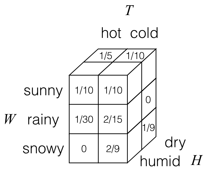
What happens when we have more than two random variables? Let’s build on our earlier example and suppose that in addition to weather W and temperature T, we also had a random variable H for humidity that takes on values in the alphabet {dry, humid}. Then having a third random variable, we can draw out a 3D joint probability table for random variables W, T, and H. As an example, we could have the following:

Here, each of the cubes/boxes stores a probability. Not visible are two of the cubes in the back left column, which for this particular example both have probability values of 0.
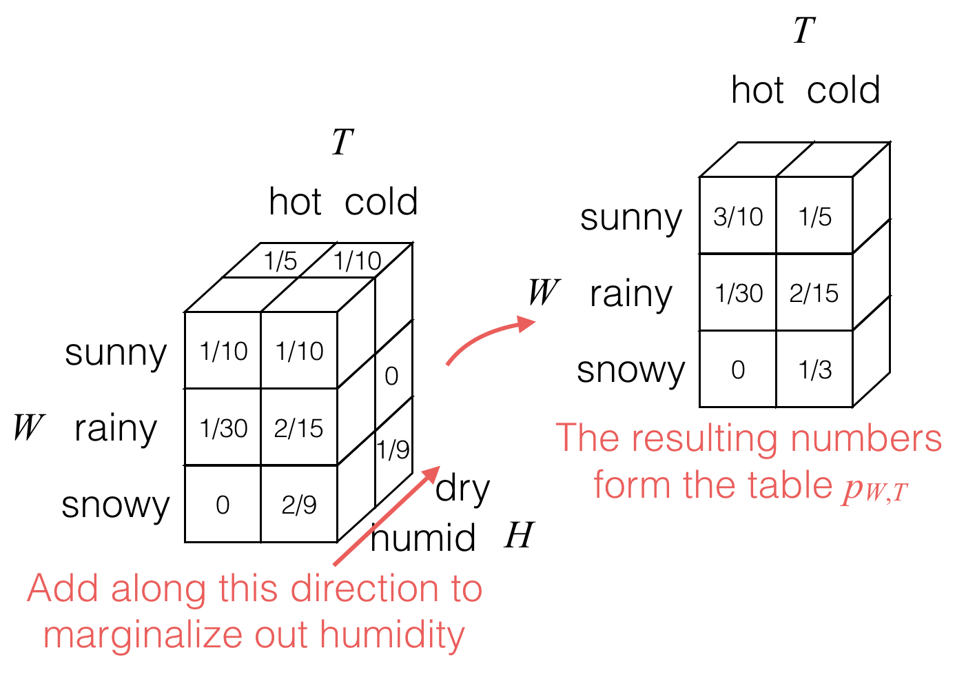
Then to marginalize out the humidity H, we would add values as follows:

The result is the joint probability table for weather W and temperature T, shown still in 3D cubes with each cube storing a single probability.
As an equation:
pW,T(w,t)=∑hpW,T,H(w,t,h).
In general, for three random variables X, Y, and Z with joint probability table pX,Y,Z, we have
pX,Y(x,y)=∑zpX,Y,Z(x,y,z),pX,Z(x,z)=∑ypX,Y,Z(x,y,z),pY,Z(y,z)=∑xpX,Y,Z(x,y,z). Note that we can marginalize out different random variables in succession. For example, given joint probability table pX,Y,Z, if we wanted the probability table pX, we can get it by marginalizing out the two random variables Y and Z:
Even with more than three random variables, the idea is the same. For example, with four random variables W, X, Y, and Z with joint probability table pW,X,Y,Z, if we want the joint probability table for X and Y, we would do the following:
pX,Y(x,y)=∑w(∑zpW,X,Y,Z(w,x,y,z)).
If we marginalize out Z first and then Y, or if we marginalize out Y first and then Z, we get the same answer for the probability table
CONDITIONING: RANDOMNESS OF A VARIABLE GIVEN THAT ANOTHER VARIABLE TAKES ON A SPECIFIC VALUE (COURSE NOTES)
When we observe that a random variable takes on a specific value (such as W=rainy from earlier for which we say that we condition on random variable W taking on the value “rainy”), this observation can affect what we think are likely or unlikely values for another random variable.
When we condition on W=rainy, we do a two-step procedure; first, we only keep the row for W corresponding to the observed value:

Second, we “normalize” the table so that its entries add up to 1, which corresponds to dividing it by the sum of the entries, which is equal to pW(rainy) in this case:

Notation: The resulting probability table pT∣W(⋅∣rainy) is associated with the random variable denoted (T∣W=rainy); we use “∣” to denote that we’re conditioning on things to the right of “∣” happening (these are things that we have observed or that we are given as having happened). We read “T∣W=rainy” as either “T given W is rainy” or “T conditioned on W being rainy”. To refer to specific entries of the table, we write, for instance,
pT∣W(cold∣rainy)=P(T=cold∣W=rainy)=45.
In general:
Conditioning: Consider two random variables X and Y (that take on values in the sets X and Y respectively) with joint probability table pX,Y (from which by marginalization we can readily compute the marginal probability table pY). For any x∈X and y∈Y such that pY(y)>0, the conditional probability of event X=x given event Y=y has happened is
pX∣Y(x∣y)≜pX,Y(x,y)pY(y).
For example,
pT∣W(cold∣rainy)=pW,T(rainy,cold)pW(rainy)=21516=45.
Computational interpretation: To compute pX∣Y(x∣y), take the entry pX,Y(x,y) in the joint probability table corresponding to X=x and Y=y, and then divide the entry by pY(y), which is an entry in the marginal probability table pY for random variable Y.