import matplotlib
import numpy as np
import matplotlib.cm as cm
import matplotlib.mlab as mlab
import matplotlib.pyplot as plt
%matplotlib notebook
matplotlib.rcParams['xtick.direction'] = 'out'
matplotlib.rcParams['ytick.direction'] = 'out'
Value function is optimal objective value, objective function evaluated at $\bar x$
$$v = F(\bar x(\theta), \theta)$$since $\bar x$ is a function of $\theta$, the total derivative of $F$ with respect of $\theta$ by chain rule will be
$$d F(\bar x(\theta), \theta) = \underbrace{F_{\bar x}(\bar x(\theta), \theta) d \bar x(\theta)}_{\text{Indirect effcet}} + \underbrace{F_{\theta}(\bar x(\theta), \theta) d \theta}_{\text{Direct effect}} \tag 1 $$
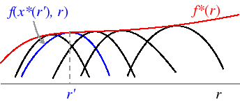
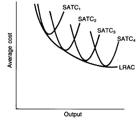
ref: http://www.g-feed.com/2014/06/adaptation-with-envelope.html
http://mathforum.org/mathimages/index.php/Envelope

ref:
https://www.slideshare.net/FarzadJavidanrad/specific-topics-in-optimisation
• Objective Function: A function which is going to be optimized.
• Decision Variables: The independent (or explanatory) variables in a model.
• Optimal Values: Maximum or minimum values of variables in a model..
• The envelope theorem focus on the relation between the optimal value of the dependent variable in a particular function and the parameter(s) of that function.
How the optimal value does change when a parameter (or one of parameters of the model) changes?
ref: https://www.slideshare.net/YosukeYasuda1/advanced-microeconomics-lecture-slides
For an optimization problem without constraint, the F.O.C is
$$ F_{\bar x}(\bar x(\theta),\theta) = 0 \tag 2 $$then plug $(2)$ into $(1)$
$$d F(\bar x(\theta), \theta) = + \underbrace{F_{\theta}(\bar x(\theta), \theta) d \theta}_{\text{Direct effect}} $$the indirect effect is $0$, and only direct effect.
For an optimization problem with constraint, the F.O.C is
$$ F_{\bar x}(\bar x(\theta), \theta) - \lambda G_{\bar x}(\bar x(\theta), \theta) = 0 \tag 3 $$here $\lambda$ can be a vector,
and for a F.O.T.S of $G( \bar x(\theta) + d \bar x(\theta), \theta + d \theta )$
$$G( \bar x(\theta) + d \bar x(\theta), \theta + d \theta ) = G( \bar x(\theta) , \theta ) + G_{ \bar x(\theta)} d\bar x(\theta)+ G_{\theta} d \theta $$since the constraints are still binding before perturbation and after perturbation,
$$G( \bar x(\theta) + d \bar x(\theta), \theta + d \theta ) = G( \bar x(\theta) , \theta )$$then
$$G_{ \bar x(\theta)} d\bar x(\theta) = - G_{\theta} d \theta \tag 4 $$Plug $(3)$ and $(4)$ into $(1)$, we have
$$ d F(\bar x(\theta), \theta) = \underbrace{- \lambda G_{\theta} d \theta}_{\text{Indirect effcet}} + \underbrace{F_{\theta}(\bar x(\theta), \theta) d \theta}_{\text{Direct effect}} $$factor out the $d \theta$,
$$d F(\bar x(\theta), \theta) = (\underbrace{- \lambda G_{\theta} }_{\text{Indirect effcet}} + \underbrace{F_{\theta}}_{\text{Direct effect}}) d \theta $$The indirect effect of $\theta$ on $F$ equals to the direct effect of $\theta$ on $G$ times $\lambda$,
since F.O.C of Lagrangean is
$$ L_{\theta} = F_{\theta} - \lambda G_{\theta} $$so
$$ \frac{dv}{d \theta} = \frac{dF(\bar x(\theta), \theta)}{d\theta} = \frac{dL}{d\theta} $$If I want to see how utility at its optimal level changes when wealth changes, I can simply differentiate this equation with respect to wealth explicitly:
$V_3=λ$ - so the marginal utility of wealth is simply the Lagrange multiplier.
The relationship between indirect utility and expenditure is from the 'duality' between the two. The reason why $V(p,e(p,u))=w$ stems from the fact that the optimal arguments for both will be equivalent when the value of utility achieved in the utility max problem is the same utility level that we set as $U= \bar u$ in the expenditure minimization problem.
Comparative Static Analysis
envelope theorem
https://mjo.osborne.economics.utoronto.ca/index.php/tutorial/index/1/mee/t
Proposition (Envelope theorem for an unconstrained maximization problem) proof Let f be a function of $n + k$ variables, let r be a $k$-vector, and let the n-vector $x^*$ be a maximizer of $f(x, r)$. Assume that the partial derivative $f'n+h(x*, r)$ (i.e. the partial derivative of $f$ with respect to $rh$ at $(x*, r))$ exists. Define the function $f*$ of $k$ variables by
$$f*(r) = maxx f(x, r) for all r.$$If the partial derivative f*h'(r) exists then
$$f*h'(r) = f'n+h(x*, r).$$This result says that the change in the maximal value of the function as a parameter changes is the change caused by the direct impact of the parameter on the function, holding the value of x fixed at its optimal value; the indirect effect, resulting from the change in the optimal value of x caused by a change in the parameter, is zero.
Example Consider the problem studied at the start of this section, in which a firm can produce output, with price p, using a single input, with price w, according to the production function f. The firm's profit when it uses the amount x of the input is $π(x, (w, p)) = pf(x) − wx$, and its maximal profit is
$$f^*(w, p) = p f(x^*(w, p)) − wx^*(w, p),$$where $x*(w, p)$ is the optimal amount of the input at the prices (w, p). This function $f^*$ is known as the firm's profit function. By the envelope theorem, the derivative of this function with respect to p is the partial derivative of π with respect to p evaluated at $x = x^*(w, p)$, namely $f(x^*(w, p))$.
In particular, the derivative is positive: if the price of output increases, then the firm's maximal profit increases. Also by the envelope theorem the derivative of the firm's maximal profit with respect to w is $−x^*(p, w)$.
(This result is known as Hotelling's Lemma, after Harold Hotelling, 1895–1973.) In particular, this derivative is negative: if the price of the input increases, then the firm's maximal profit decreases.
A consequence of Hotelling's Lemma is that we can easily find the firm's input demand function $x*$ if we know the firm's profit function, even if we do not know the firm's production function: we have $x^*(p, w) = −π^* w'(p, w) for all (p, w)$, so we may obtain the input demand function by simply differentiating the profit function.
Proposition (Envelope theorem for constrained maximization problems) Let $f$ and $g1, ..., gm$ be continuously differentiable functions of $n + k$ variables, with m ≤ n. Suppose that for all values of the k-vector r the problem $max_x f(x, r)$ subject to $g_j(x, r) = 0 for j = 1, ..., m$, where x is an n-vector, has a unique solution, which is differentiable in r. Denote this solution $x^*(r)$ and define the function $f^*$ of $k$ variables by
$$f*(r) = maxx f(x, r) subject to gj(x, r) = 0 for j = 1, ..., m.$$Suppose that the rank of the $m × n$ matrix in which the $(i, j)$th component is $(∂gj/∂xi)(x^*(r), r)$ is m. Define the function L by
$$L(x, λ, r) = f(x, r) − ∑^m_{j=1}λ_{j}g_{j}(x, r) for every (x, λ, r),$$where $x$ is an n-vector, $λ$ is an m-vector, and $r$ is a k-vector. Then
$$f*h'(r) = L'_{n+m+h}(x*(r), λ(r), r) for h = 1, ..., k,$$where $λ(r) = (λ_1(r), ..., λ_m(r))$ and $λ_j(r)$ is the value of Lagrange multiplier associated with the jth constraint at the solution of the problem.
Example
Consider a utility maximization problem:
$$max_x u(x) subject to p·x = w.$$where x is a vector (a bundle of goods), p is the price vector, and w is the consumer's wealth (a number). Denote the solution of the problem by x(p, w), and denote the value function by v, so that $$v(p, w) = u(x(p, w)) for every (p, w).$$ The function v is known as the indirect utility function. By the envelope theorem for constrained maximization problems we have $$(∂v/∂pi)(p, w) = −λ^(p, w)x_i^(p, w)$$ (since u does not depend independently on p or w) and $$(∂v/∂w)(p, w) = λ^(p, w).$$ Thus $$\frac{(∂v/∂pi)(p, w)}{(∂v/∂w)(p, w)} = −x_i^(p, w).$$
That is, if you know the indirect utility function then you can recover the demand functions. This result is known as Roy's identity (after René Roy, 1894–1977).
https://economics.stackexchange.com/questions/13267/understanding-the-envelope-theorem
$$V(p_x,p_y,w)=U(x(p_x,p_y,w), y(p_x,p_y,w))+\lambda(p_x,p_y,w)[w-p_x-p_y]$$import sympy as sym
sym.init_printing()
x,y,z = sym.symbols('x y z')
a,b,c = sym.symbols('a b c', positive = True)
f, g, h = sym.symbols('f g h', cls=sym.Function)
f = sym.Function('f')
g = sym.Function('g')(x)
x1,x2,lam = sym.symbols('x_1 x_2 lambda', positive = True)
3b
F = a*x1+4*x2
F
G = x1**0.25*x2**0.75
c = 10
G
L = F + lam*(c-G)
L
L1 =sym.diff(L, x1)
L1
L2=sym.diff(L, x2)
L2
Llam =sym.diff(L, lam)
Llam
sol1=sym.solve([L1,L2,Llam], x1,x2, lam,dict=True)
sol1
La = sym.diff(L,a)
La
La.subs({x1:sol1[0][x1]})
3e
F = 2*x1+3*x2
F
G = 2*x1**2+a*x2**2
c = 10
G
L = F + lam*(c-G)
L
L1 =sym.diff(L, x1)
L1
L2=sym.diff(L, x2)
L2
Llam =sym.diff(L, lam)
Llam
sol1=sym.solve([L1,L2,Llam], x1,x2, lam,dict=True)
sol1
La = sym.diff(L,a)
La
La.subs({lam:sol1[0][lam],x2:sol1[0][x2]})
## 3f
L = 2*x1+ 3*x2 + lam*(10-a*x1**2 -5*x2**2)
L
L1 =sym.diff(L, x1)
L1
L2=sym.diff(L, x2)
L2
Llam=sym.diff(L, lam)
Llam
sol2 =sym.solve([L1,L2,Llam], x1,x2, lam,dict=True)
sol2
La=sym.diff(L, a)
La
La.subs({lam:sol2[0][lam],x1:sol2[0][x1]})
sym.simplify(La.subs({lam:sol2[0][lam],x1:sol2[0][x1]}))
sol1[0][x1]
sym.simplify(sol1[0][x1])
sol1[0][lam]
delta = 0.025
x = np.arange(-3.0, 3.0, delta)
y = np.arange(-2.0, 3.0, delta)
X, Y = np.meshgrid(x, y)

bc = 2-x

Z = X**0.5*Y**0.5


# Create a simple contour plot with labels using default colors.  The
# inline argument to clabel will control whether the labels are draw
# over the line segments of the contour, removing the lines beneath
# the label
plt.figure()
BL = plt.plot(x, bc, '-r')
CS = plt.contour(X, Y, Z)
plt.clabel(CS, inline=1, fontsize=10)
plt.title('Contour curve/IC and Budget line')
plt.xlim(0,3)
plt.ylim(0,3)